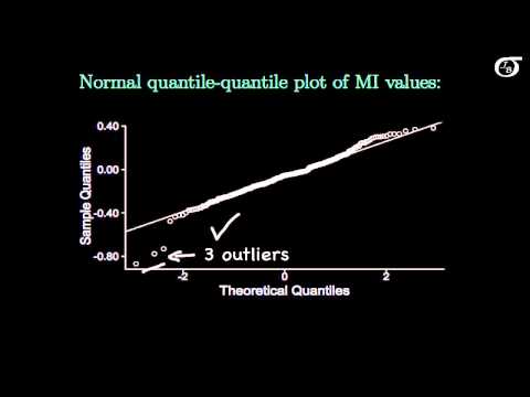
Let's take a look at an example of a t test for the population mean mu. Are healthy normal sleepers able to accurately state the next morning how much sleep they got the night before? A study investigated this question on 288 normal sleepers. By normal, we mean not insomniacs, people who tended to get a regular night's sleep. The individual slept for a night, had technology measure the actual amount of sleep and then were asked the next mornin 30how much sleep do you think you got the night before? Based on this, a misperception index was recorded for each person. The further the estimated amount to sleep they ot was from the actual amount of sleep, the further the misperception index would be from 0. I'm not going to go into the details of exactly what that Misperception Index (MI) represents, but if an individual correctly estimated their total sleep time, MI would equal 0. If an individual underestimated their total sleep time, MI would be greater than 0. And the more they underestimated it, the greater MI would be. And if an individual overestimated their total sleep time, MI would be less than 0. A natural question that arises i 20is there strong evidence that the true mean MI differs from zero in normal sleepers? So we may wish to test the null hypothesis that mu is equal to 0, where mu is the true mean MI value for normal sleepers. Here we're interested in a difference from zero in either direction, we want to see whether the true mean MI value differs from zero. We'd like to know whether it's greater than or whether it's less than 0, so we're going to test the null hypothesis against this alternative hypothesis that mu is different from 0. The results for the 288 sleepers in the sleep study were a sample mean of -0.06 and a sample standard deviation of 0.183. Let's plot our data and see what that looks like. Here's a boxplot of the 288 MI values, and I've put in a red line indicating the hypothesized value of mu at 0. The sample mean was -0.064, which is around there somewhere, X bar was -0.064, and what we're going to do with our test is see if this observed difference here is statistically significant. It doesn't look like there's a big difference there, but the sample size is rather large, so let's see what the test has to say. Another thing to take note of here is that we have 3 outliers on the low end, and outliers can influence the results of a t test. We'll take a look at that a little later on. The t test assumes that we are sampling from a normally distributed population. For a sample size as large as the one that we have here, 288 observations, the normality assumption is not that important. But it can still be informative to plot a normal quantile quantile plot and have a look. One of the things we might notice right away is these 3 small outliers appear here as well. Other than that, the plot is a reasonably straight line, so I'm going give this the qualified check mark and say that it's reasonable to use the t procedures here. These 3 outliers should give us some pause, but for a sample size of 288, they're probably not going to have too much of an effect, but let's investigate that later on. Recall again that we're testing the null hypothesis that mu=0 against a two-sided alternative. The standard deviation of 0.18 was based on the 288 observations in the sample, and since the standard deviation is based on sample data, we should be using a t statistic, this t statistic. And this is equal to, in this case, the sample mean of -0.064 minus the hypothesized value of 0, divided by the standard deviation over the square root of n. And this works out to -5.935. and the p-value is going to come from the t distribution with the appropriate degrees of freedom. And for the one-sample problem the degrees of freedom are n-1, or in this case 287. Here's a t distribution with 287 degrees of freedom. With 287 degrees of freedom the t distribution is very close to the standard normal distribution, so if you used the standard normal distribution instead, you wouldn't be too far off the mark. But it's still slightly better to use a t distribution with this appropriate degrees of freedom. The observed value of our test statistic is over here somewhere, at -5.935. The alternative hypothesis is two-sided which means that the p-value is the area in the tail beyond the test statistic, doubled. Or in other words, the p-value is double the area to the left of -5.93 under a t distribution with 287 degrees of freedom. From the plot we can see that there is very little area to the left of the observed value of the test statistic, and so our p-value is going to be very small. Using software we can find out that the p-value is equal to 8.5 times 10^-9. If we didn't have access to software, and we could only use a t table, we'd have to say something lik he p-value is very close to zero. What does that mean? We don't have a significance level given to us, but we don't need one to come up with a reasonable conclusion. This is a very tiny p-value, giving very very very strong evidence against this null hypothesis and in favour of this alternative. So we have a very strong evidence that the true mean differs from 0. Also note that the test statistic is way out here in the left tail of the distribution, Indicating that we have evidence that the true mean is actually less than 0. And so we have very strong evidence, with our two-sided p-value of approximately 8.5 times 10^-9, that the true mean MI for normal sleepers is less than 0. In slightly loose terms, normal sleepers tend to overestimate how much sleep they got the night before. An MI value less than zero indicated that the individual overestimated how much sleep they got. Normally we carry out the analysis on a computer and let the software do the number crunching for us. Here's the output from the statistical software R. And we see our t value up here, the appropriate degrees of freedom, and the p-value. One thing to take note of here is that the sample size was rather large at 288, so even though we had a sample mean that was fairly close to zero we found a highly statistically significant difference. It can also be informative to report the appropriate confidence interval as well as the results of the hypothesis test and let experts decide whether that's a meaningful difference. In fact the authors of the study that inspired this example felt that the MI values were actually quite close to zero for normal sleepers. Let's take a quick look again at this boxplot, and these 3 outliers we had down here. What effect did those outliers have on the analysis? Let's take a look at the results of the t-test with and without the outliers. The first bit is from the output that we just looked at, with all observations included, and the second bit is with those 3 outliers removed. And our t statistic changes a little bit and our p-value changes a little bit, but overall the conclusions remain pretty much the same. Since our conclusions did not change a great deal when those observations were removed, we can feel okay about reporting the results with all observations included. If the results changed a great deal with the observations were removed, then it's much more problematic. We should not be willing to simply throw observations out because we don't like them in there, but we also don't like our conclusions to rest entirely on one or a few obsevations. So it can be a difficult situation to deal with, but that's another talk for another day.